
Chris Sparrow, head of research
When we analyse our trading performance using transaction cost analysis (TCA), we need to realise there are things that are not in our control, like the liquidity available in the market, and things that are in our control, like how we interact with the market – our trading strategy. The trading strategy describes the prices and volumes we obtained in the market and include the venue distribution and the time distribution of volume executed passively and actively, lit and dark, etc.
The point of TCA is to uncover insights in our execution data. These insights can shed light on how to best model market impact of our orders along with many other use cases. Other use cases include comparing how different algos trade different securities, how stable the trading strategies are and many others.

Melinda Bui, director of trading analytics
We can use machine learning (ML) algorithms to help us extract these insights from our historical set of order data. In this article we explain a key part of the process of applying ML to TCA – applying our domain knowledge to our database of client orders to create features that help us get the most out of the ML algos.
The trading strategy is often dictated by the type of algo employed, along with specific parameters that modify the default strategy. Depending on our reasons for trading and the liquidity characteristics of the stock, we may want to modify our trading strategy. Since we measure the performance of each order using various benchmarks, we can analyse how performance varies with trading strategy.
When we talk about a trading strategy, we generally mean the volume profile of our order as a function of time. There are other components related to venue selection (eg: whether dark pools are accessed, etc…) which can also be measured to understand the way our order interacted with the market. We can then take these measurements and create analytics, or features, to describe the trading strategy.
We are particularly interested in the trading strategy because that is how we interacted with the market and so we expect that for our primary use case, measuring market impact, the degree of impact will depend in part on our trading strategy.
To put this another way, we want to be able to do scenario analysis using our pre-trade market impact model, and we want to see how our expected impact changes for different trading strategies. We use our past data to ‘learn’ how the impact varies with strategy and then take the resultant model to use in the scenario analysis. This is why having a large repository of order data is so crucial. We need to see a lot of outcomes to be able to properly train, test and validate a model.
We want to create features (AKA analytics) that can distil a large amount of data into a smaller amount of data. We can also enrich the data by applying our domain knowledge. We do this by aggregating and combining the data into features that describe the business process we want to model. As an example, we may want to separately aggregate all of the volume from liquidity removing trades and liquidity providing trades to compute a ratio of active to total volume.
If we want to be able to model how our orders interact with the various order books that make up the market, we need to prepare the data, both market data and our order data.
Rather than pass every new order book update to the model, we instead compute time-weighted liquidity metrics, such as depth of liquidity on a scale of minutes rather than microseconds. This process turns highly granular order book messages into aggregated analytics (features) that describe liquidity in a more macro way. We can apply similar approaches to our order data.
Engineering order features for our model starts off with a question we want to answer: What is the relationship (if any) between the trading strategy and the implementation shortfall of our order?
The first task is to try and come up with the appropriate features that we think will help us identify a relationship. It can help to look at a volume profile that shows aggregated volume binned into 15-minute intervals. We can also show the colour of the volume done actively versus passively. We may even want to show the venues where we got the volume (but that would make the chart very hard to read).
The trading strategies that could be employed range from trading most of the volume close to the start of the order to trading most of the volume near the end of the order. Other strategies would trade their volume at a more consistent pace.
One feature we can try is to compute the time-weighted unfilled portion of the order. If most of the volume is traded at the beginning of the order, then the pace of trading slows down as the order proceeds. This proposed feature would have a small value because most of the order volume is executed in a short amount of time at the beginning of the order. If most of the volume were traded near the end of the order, the feature would have a large value. A more symmetric strategy, like a VWAP, would have a value close to 50% since the volume profile is close to being symmetric in time.
Figure 1 shows some examples of trading strategy volume profiles along with the time-weighted average unfilled portion of the order. We will call the value of the proposed feature exposure. The exposure is the area under the curve shown in Figure 1 (below).
When we examine the trading profiles of various strategies, we also notice that some of the strategies may be symmetric, but they don’t trade consistently through the lifetime of the order. There are some periods where there is a lot more volume and other periods where there may be no volume. We can create another feature to measure this by fitting the time-weighted unfilled portion of the order with a linear model. We can define a ‘roughness’ feature by computing the variance of the difference between the model and the data. If the trading strategy is smooth, like a VWAP in a liquid security, then the ‘roughness’ will be low, whereas in other strategies that may be symmetric, but not consistent, the ‘roughness’ will be high.
There are several other features that we can construct to help describe the trading strategy. The key is to have as few features as possible while maximising information capturing, meaning we need the important features, but we want to get rid of the superfluous features.
We can use some ML techniques to decide on which features are important, so it is better to try as many features as possible, while only keeping those with the best explanatory power.
There are other things we can use these features for. As an example, maybe we want to compare the trading strategies of two different algos, or how an algo’s trading strategy may vary for securities that have different liquidity characteristics. We don’t have to use ML to get value out of features like these, but the features are very useful if and when we decide to implement an ML program.
By computing features like these and then curating them, we can build up libraries of analytics that can help us not only apply ML algorithms to find patterns in our data, but also to compare how those analytics vary through time as market structure evolves.
It is important to keep in mind that when our order is being executed in the market, the market doesn’t care if the algo had a label, it cares instead about the orders that interact with the order book and potentially become fills.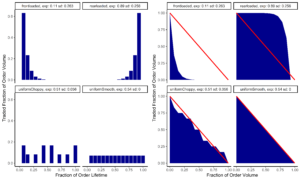
Figure 1: The set of four charts on the left show 4 trading strategies. The top left shows a front-loaded strategy where volume is traded quickly at the beginning of the order and then the pace of trading slows down as the order progress. The top right strategy shows a back-loaded strategy where the pace of trading accelerates as the order is completed – like trading a ‘Close’ strategy. The bottom right strategy is uniform in time where trading occurs at a constant pace and the volume profile is symmetric in time. The bottom left strategy is symmetric but trades at a variable pace.
The charts on the right show the unfilled portion of the order over time. The area under the curve represents the ‘exposure’ of the unfilled shares to opportunity risk. The top left has a low value, the top left has a high value and the bottom row are both intermediate. The bottom right shows a smooth profile while the bottom right is rougher. Our second metric, ‘roughness’ characterises the difference of the trading strategy from a smooth strategy.